Geological mapping in the Owaria-Touno area, Japan

Preface

1 Outline of Geology (Link)

2 Geology (Link)

3 Geological mapping (Link)

4 Practice course (Link)

5 Radiation dose survey (Link)

6 Water quality survey (Link)

7 Geographical Information System (Link)

Preface

This is prepared for a person who wants to study geological mapping by oneself. Model field routes are selected from the Owari-Touno area. Some examples of mapping are shown in the following chapters.

--------------------

1. Outline of Geology

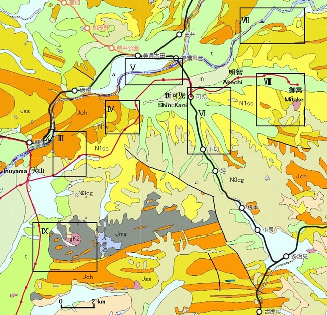
Fig. 1-1 Geological map

The areas of III to X are the guide maps in Geologic guide for Hiromi Rail Line.

Geologic guide for HIROMI Rail Line,　http://y95480.g1.xrea.com/hiromi_line_geology.htm

Cenozoic; a, Alluvium; t, Terrace deposits; N3cg, Sandy gravel; N1ss, Miocene sandstone and mudstone; N1v, Miocene tuffaceous sandstone and conglomerate

Mesozoic; gK, Granite; Jss, Sandstone and mudstone; Jms, Mudstone; Jch, Chert

Geologic age	Geologic division	Abbr.	Lithology	Geological history
Quaternary Holocene Pleistocene	Alluvium Gentle slope deposits Mudflow deposits Terrace deposits	(a) (s) (m) (t)	Gravel, sand and mud Gravel, sand and mud Gravel, scoria and mud Gravel and sand	Alluvial plain Volcanic detritus Terrace
Neogene Pliocene Miocene	Toki Sandy Gravel F. Nakamura Formation Hachiya Formation	(N3cg) (N1ss) (N1v)	Gravel and sand Sandstone and mudstone Pyroclastic rocks	Terrestrial Terrestrial Terrestrial volcanics
Paleogene
Cretaceous	Granite	(gK2)	Granitic rocks	Felsic magmatism
Jurassic Triassic Permian	Mino Complex Kamiaso Unit	(Jms) (Jss) (Jsi) (Jch)	Mudstone with clasts Sandstone and mudstone Siliceous mudstone Chert	Melange Sedimentation Sedimentation Sedimentation

Based on Yoshida and Wakita (1999).

To Top (Link)

------------------------

2．Geology

2．1 General remarks

The district covers the border area of Aichi and Gifu Prefectures and is topographically occupied by the Mino Mountains in northern half and the Nobi Plain in southern half. The Kiso River runs from northeast to southwest in northern area.

The Mino Mountains consist of Mino Sedimentary Complex and the Nobi Plain is floored with Middle to Late Pleistocene and Holocene sediments. Small granitic bodies in Late Cretaceous age are intruded into the Mino Complex. The Early Miocene Hachiya and Nakamura Formations and Early Pliocene Toki Sandy Gravel Formation overlie the complex in the hilly region and underlie Pleistocene and Holocene deposits in the Nobi Plain.

2．2 Geology

Mino Sedimentary Complex (Jch, Jsi, Jss, Jms)

The Mino Sedimentary Complex of Jurassic to earliest Cretaceous age is the oldest formation in this guide area. The complex in this guide is tectonically characterized by the assemblages of the tectonic slices that are composed of siliceous claystone (Late Permian to Early Triassic), bedded chert (Middle Triassic to Early Jurassic), siliceous mudstone (Middle Jurassic), alternation of sandstone and mudstone, and massive sandstone (Middle to Late Jurassic).

Cretaceous Granite (gK2)

The granitic rocks crop out south of the Mitake station and east of the Haguro station. They may belong to Cretaceous Naegi Granite, Sanyo Zone. They may be petrographically granite to granodiorite. K-feldspar phenocryst shows ENE-WSW direction and gentle plunge in lineation structure in the Mitake area.

Upper Cenozoic (N1v, N1ss, N3cg, t, s, a)

The upper Cenozoic in this guide are divided into the Lower Mizunami Group, the Lower Pliocene Tokai Group, Middle to Late Pleistocene sediments (mostly terrace deposit), and Holocene alluvial sediments.

The Mizunami Group is divided into the Hachiya and Nakamura Formations in ascending order. The Hachiya Formation consists chiefly of andesitic pyroclastic rocks. The U-Pb age in zircon is 22.38±0.17Ma in the lowest part of the formation. The Nakamura Formation is mostly composed of interbedded sandstone and mudstone. These formations are of non-marine origin.

The upper sediments of the Tokai Group are alluvial fan origin and called the Toki Sandy Gravel Formation. It is composed of gravel and sandy gravel. Zircon in this formation gives 3.94±0.07Ma of U-Pb age and 3.97±0.39Ma of fission track age.

Middle to Late Pleistocene sediments can be divided into gravelly terrace deposits and mudflow deposits. The terrace deposits are subdivided into a few deposits in the Seamless Geologic Map of GSJ but will be described as only terrace deposits in this guide. The mudflow deposits may be originated from the Kiso-Ontake Volcano. Holocene alluvial sediments are made up of gravel, sand and mud. Most of them are valley bottom plain deposits.

2．3 Mineral resources

Manganese ore is embedded in the chert of the Mino Complex. Small manganese mines were once operated in the mapped area and were all closed by the end of the 1970’s.

---------------------------

3. Geological mapping

The geologic map shows the distribution of rocks and strata with a color and a design on the topographical map. It is a required for mineral prospecting, engineering and disaster prevention.

Preparations for a geological survey: Carry the rucksack containing some materials on your back for being both hands free. The tools for geological mapping are a map, a notebook, writing implements, a hammer, a clinometer and a loupe (or insect glasses). A plastic bag or an old newspaper may be useful for sample collections.

A geological survey: Observe geological feature of strata and rocks. You write down the location name in the notebook and the location point on the map. You write latitude and longitude if you can know. You should measure strike and dip of strata of a sedimentary rock.

Strike and dip: You will distinguish the border of the stratum in difference of grain size and composition. The boundary surface is called a stratification plane. The direction, an intersection of the stratification plane and the horizontal plane is a strike and the angle between two planes is dip.

A geologic map: If there are many strata data, you can draw a geological feature border by freehand. Mostly you presume a geologic border geometrically.

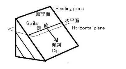
Fig. 3-1 Strike and dip of the strata

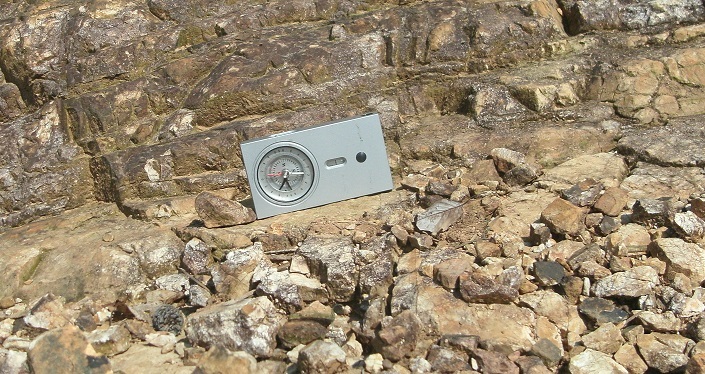
Fig. 3-2 Dip of strata.

To top (Link)

-----------------------

4. Geologic mapping courses

4.1 Strata

Area; Kani-Forest Park

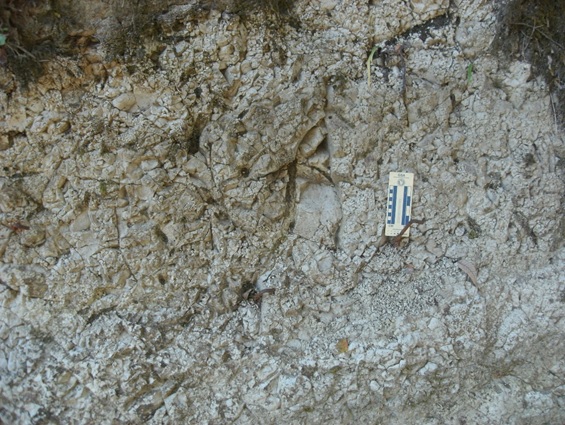
Fig. 4-1-1 Mudstone

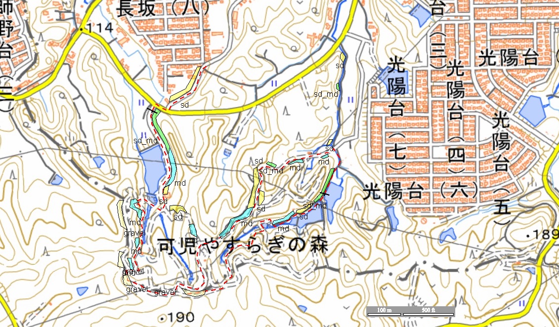
Fig. 4-1-2 Route map

Legend; sd, Sandstone; md, Mudstone; sd_md, Sandstone and Mudstone; gravel, Gravel; red dash line, mapping route.

Upper strata are appearing from the Car Park sites to southward. Gravel layer appears on the top of the hill, which shows unconformable relation over Miocene sandstone and mudstone. The following is schematic idea.

(North) <‐‐‐‐‐‐‐‐‐‐‐> (South)

Gravel　(unconformity)

Mudstone

Sandstone

Sandstone and Mudstone

Sandstone

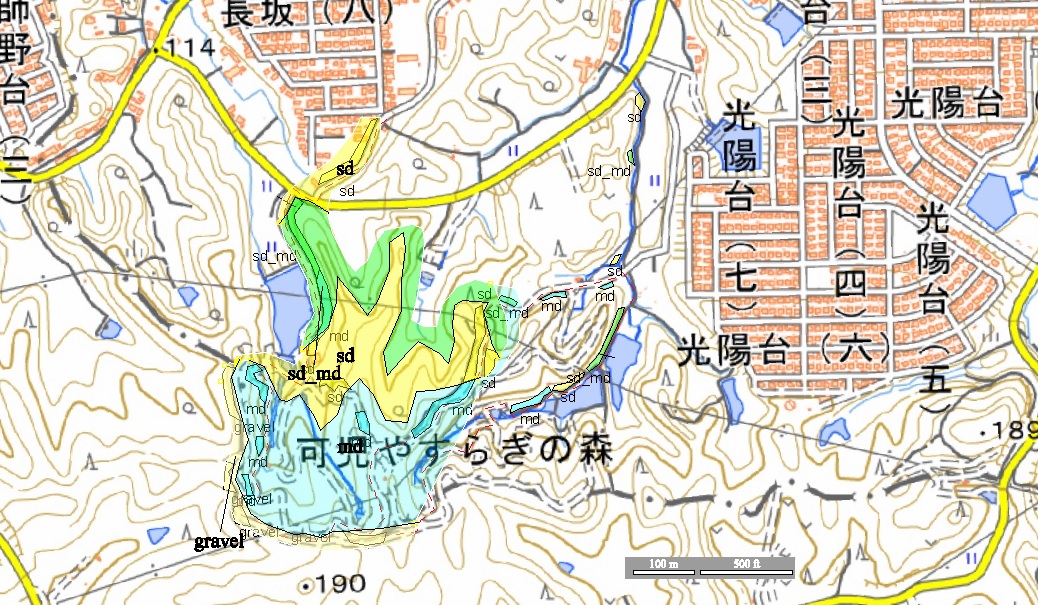
Fig. 4-1-3 Geologic map

Legend; sd, Sandstone; md, Mudstone; sd_md, Sandstone and Mudstone; gravel, Gravel.

A geologic boundary is almost parallel to contour lines due to low dip of a stratum.

4.2 Fold structure

Bent rock strata is fold.

Anticline; A fold of rock layers that is convex upwards.

Syncline; A fold of rock layers that is convex downwards.

Area; West of Tajimi and Koizumi stations.

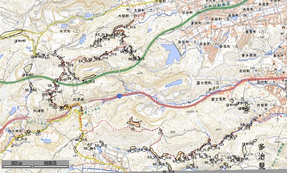
Fig. 4-2-1 Route map

Legend; ch, Chert; ss_ms, Mesozoic Sandstone and Mudstone; gravel, Gravel.

North part shows north to northwest ward dipping of the strata

South part shows south to southeast ward dipping of the strata.

Therefore an anticline structure is deduced in the midst of these two parts.

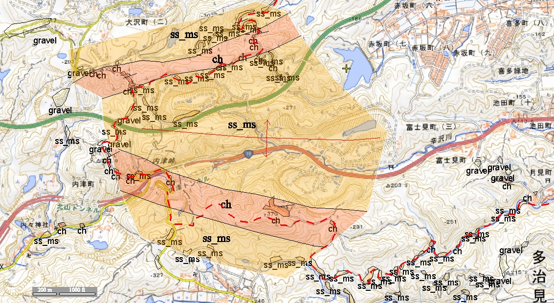
Fig 4-2-2 Geologic map　

Legend; ss_ms, Sandstone and Mudstone; ch, Chert; red line with arrow symbol, Anticline axis.

Micro-folding

Micro-folding occurs in chert around Mt. Ikeda-Fuji.

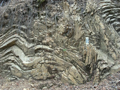
Fig. 4-2-3 Micro-folding　

Near Mt. Ikeda-Fuji.

4.3 Deducing geological structure from strata distribution

Geological structure can be deduced from the distribution of strata.

Area; Kasugai three tops

Kasugai three tops are Mt. Dojyu-san, Mt. Otani-san, and Mt. Miroku-san from south to north.

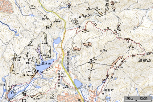
Fig. 4-3-1 Route map

Legend; ls, Limestone; ch, Chert; ss_ms, Sandstone and Mudstone; gr, Granite; gravel, Gravel.

Fig. 4-3-2 Geologic map around Kasugai three tops

Legend; ls, Limestone; ch, Chert; ss_ms, Sandstone and Mudstone; gr, Granite; gravel, Gravel; a_t, alluvium and terrace deposit.

Geological boundary near Mt. Dojyu-san in SE part of the map can give geological structure. The boundary crosses 350m contour. Two crossed points give a strike direction. Assume a line with a point crossed 250m contour parallel to a strike direction. Direction normal to this line is dipping direction. Distance in horizontal plane between 350m and 250m contours is 200m.

Therefore, tan D = (350 – 250)/200 = 0.5, D is dip angle.

D = 27°, dip direction is SSE.

General trend of the strata is ENE-WSW in strike and 27°SSE in dip.

To top (Link)

--------------------------

5. Radiation dose survey

Radiation dose is different in rock types. For example, dose of granites is generally higher than dose of sedimentary rocks. A dose meter for home environment is cheap and can be got in a drugstore. In this survey, “Air Counter S” is used.

Area; Tokai Natural Pass around Jokoji station, JR.

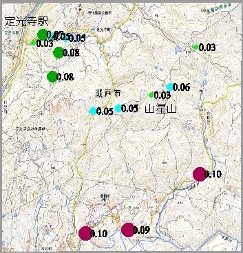
Fig. 5-1 Survey result. Date; April 20, 2024.

Unit; μSv/h.

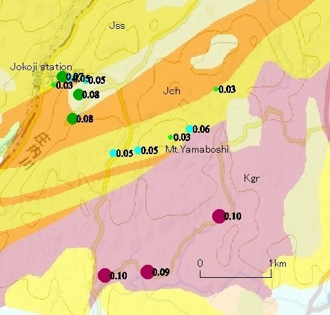
Fig. 5-2 Relationship with geology

Geologic map referred to GSJ seamless map.

Geology; Jch，Chert; Jss，Sandstone; Kgr, Granite.

Granite area shows high dose value.

To top (Link)

-----------------------

6. Water quality survey

Handy survey instruments, LAQUAtwin meters, Horiba, are used. Data of pH，conductivity (EC) and calcium ion (Ca²⁺) are shown in the following.

Example 1 Area of Owari-Fuji, Iruka-ike lake and Mt. Hongu

Map; http://y95480.g1.xrea.com/water_owari_map.jpg

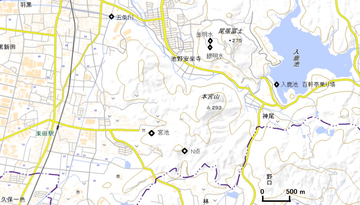
Survey result

pH

Date	River Gojogawa	Owari Fuji，Ginmei-sui	Owari Fuji，Kinmei-sui	Irukaike Pond	Mt. Hongu，N point	Mt. Hongu，Miyaike
23/1/21		7.2	7.2	6.8	7.2	7.1
23/3/4		7.3	7.4	7.1	7.4	6.9
23/5/3	7.3	7.3	7.2	7.2	7.2	6.9
23/7/30	7.1	7.2	7	7.2	7.5	6.9
23/11/23	7.4	7.6	7.5	7.2	7.3	7.3
24/3/19	6.8	7.2	7	6.9	7.2	6.7
24/6/3	7.2	7.6	7.2	7.3	7.6	7.2
24/10/26	7.7	7.7	7.6	7.6	7.6	7.1
25/03/01	7.1	7.5	7.4	7	7.6	7.3

EC μS/cm

Date	River Gojogawa	Owari Fuji，Ginmei-sui	Owari Fuji，Kinmei-sui	Irukaike Pond	Mt. Hongu，N point	Mt. Hongu，Miyaike
23/1/21		38	51	126	35	60
23/3/4		46	54	135	33	66
23/5/3	120	35	47	111	34	63
23/7/30	67	33	43	72	30	59
23/11/23	231	39	49	112	36	61
24/3/19	207	36	50	119	35	57
24/6/3	113	33	50	83	33	56
24/10/26	207	40	50	92	36	58
25/03/01	222	38	51	112	33	56

Ca ion, ppm

Date	River Gojogawa	Owari Fuji，Ginmei-sui	Owari Fuji，Kinmei-sui	Irukaike Pond	Mt. Hongu，N point	Mt. Hongu, Miyaike
23/1/21		5	7	32	5	25
23/3/4		4	7	26	4	23
23/5/3	22	3	6	18	3	15
23/7/30	25	5	11	25	4	25
23/11/23	58	5	8	26	4	25
24/3/19	61	6	10	31	5	15
24/6/3	22	3	7	14	3	12
24/10/26	46	4	7	17	3	11
25/03/01	67	5	9	22	4	10

Diagrams are drawn from the above data.

pH

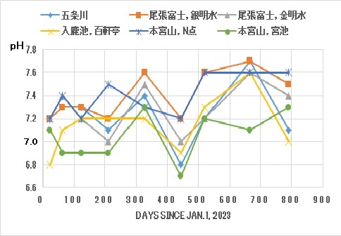
Thin Blue. River Gojo; Orange, Ginmeisui; Gray, Kinmeisui; Yellow, Irukaike pond;

Blue. Hongusan N point; Green, Hongusan Miyaike.

・Minor difference among locations, visible difference on every survey date.

EC, μSV/cm

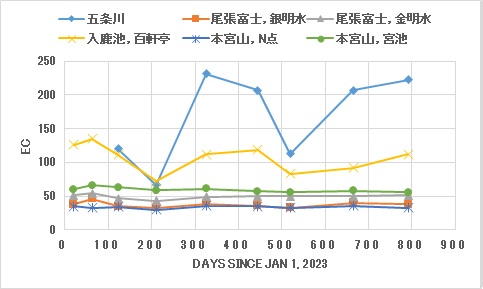
Thin Blue. River Gojo; Orange, Ginmeisui; Gray, Kinmeisui; Yellow, Irukaike pond;

Blue. Hongusan N point; Green, Hongusan Miyaike.

・Data in R. Gojo and Irukaike are visible difference among survey date.

・These two locations data are generally higher than the other locations data.

・The other four locations data are low and almost constant.

Example 2 Area around the Nagoya University of Economics

Map; http://y95480.g1.xrea.com/water_nue_map.jpg

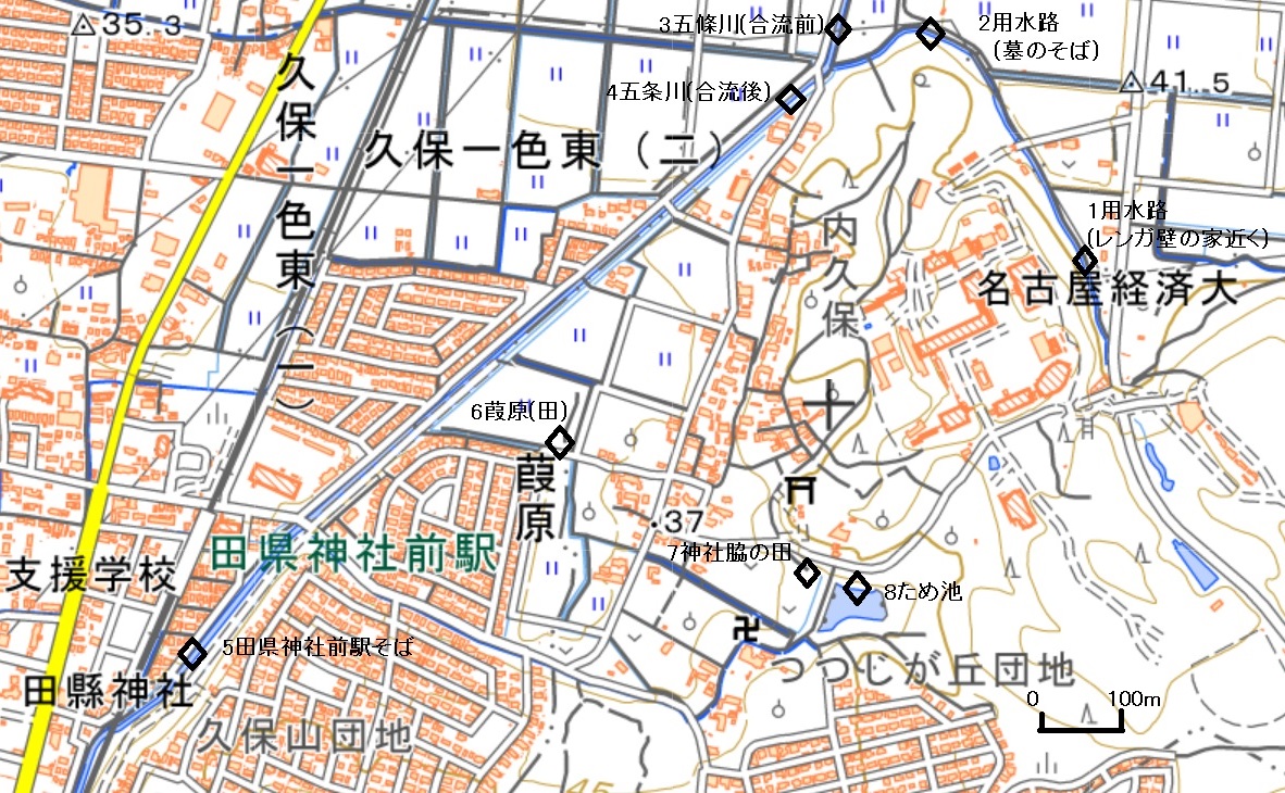
Survey result example

	1Drain	2Drain，Grave	3R.Gojo before drain confluence	4R. Gojo after drain confluence	6Rice field, Ashihara	7Rice field, Shrine	8Pond
Date	2023/6/20 PM	2023/6/20 PM	2023/6/20 PM	2023/6/20 PM	2023/6/20 PM	2023/6/20 PM	2023/6/20 PM
pH	7.0	7.5	7.5	7.4	8.0	9.4	8.2
EC (µS/cm)	166	173	139	141	211	181	78
Ca ion (ppm)	47	58	35	37	55	42	22
Water T. (℃)

Variation of pH in rice fields

	6Rice field, Ashihara	7Rice field, Shrine	8Pond
Date	2023/6/26 0805	2023/6/26 0810	2023/6/26 0815
pH	6.9	6.8	7.2

	6Rice field, Ashihara	7Rice field, Shrine	8Pond
Date	2023/6/26 1005	2023/6/26 1010	2023/6/26 1015
pH	7.3	7.0	6.8

	6Rice field, Ashihara	7Rice field, Shrine	8Pond
Date	2023/6/26 1150	2023/6/26 1155	2023/6/26 1200
pH	7.6	7.7	7.4

	6Rice field, Ashihara	7Rice field, Shrine	8Pond
Date	2023/6/26 1400	2023/6/26 1405	2023/6/26 1410
pH	7.8	8.3	7.0

	6Rice field, Ashihara	7Rice field, Shrine	8Pond
Date	2023/6/26 1555	2023/6/26 1600	2023/6/26 1605
pH	8.0	8.4	7.6

Summary of pH variation at Locality 7, 2023/6/26

Time	8:10	10:10	11:55	14:05	16:00
Minutes(8:00=0)	10	130	235	365	480
pH	6.8	7	7.7	8.3	8.4

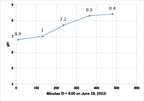
Interpretation

Phytoplankton and the alga breathe by night, and they photosynthesize in the daytime.

Breathe; Organic material　＋　O₂　→　CO₂　＋　H₂O　＋　Energy

Photosynthesize; CO₂　＋　H₂O　＋　Sun energy　→　Organic materials　＋　O₂

Carbon dioxide occurs when they breathe, and pH falls because underwater carbon dioxide increase.

Underwater carbon dioxide decreases to use carbon dioxide by the photosynthesis, and pH rises.

To top (Link)

----------------------

７　Introduction to GIS

Targets in this data processing

・Location point is defined on the map by coordination (GPS data).

・Input each point analytical data.

・Each point data is distinguished by color and/or size in the map.

7.1 Geographical map

Your map should be scanned. Coordination of some points in the map should be referred.

・Geographical map in Geographical Survey Institution

https://maps.gsi.go.jp/#6/37.640335/140.119629/&base=std&ls=std&disp=1&vs=c1g1j0h0k0l0u0t0z0r0s0m0f0

Coordination can be known in this map. Coordination of the center point (center of cross mark) can be known in Lower left part.

・If this map is not available, choose the map in the following GSI site.

https://www.gsi.go.jp/tizu-kutyu.html

7.2 GIS (Geographical Information System) soft wear

TNT mips of Microimages

Download TNT mips of Microimages

http://www.microimages.com/downloads/tntmips.htm

If we use small data size, we can use freely this soft wear.

7.3 Map Raster

The map image should be raster style.

Menu bar

[Main Image Geometric Terrain Database Script Tools]

↓(Pull down)

Display

Edit

Georeference

Process List

Import

Export

TNT atlas

Exit

Open Import.

「Select Files」

Select a file of the map.

Push “+”, then “OK”.

Next

「Import from …」

Push “Import”, then OK.

Raster map is made.

Folder, File and Object should be named.

This new raster style map runs in GIS.

7.4 Georeference

Menu bar

[Main Image Geometric Terrain Database Script Tools]

↓(Pulldown from Main)

Display

Edit

Georeference

Process List

Import

Export

TNT atlas

Exit

Open Georeference

Select the object and mark +.

「Coordination Reference System」, 「OK」

「Select georeference model」, 「OK」

「Georeference Input View」

Put + (Cross mark) to the point which was defined coordination.

Input coordination data, and push 「✔」. The other points should be also defined. Save in the file menu.

7.5 Input the point data on the map

Map will be shown.

Menu bar

[Main Image Geometric Terrain Database Script Tools]

↓(Pull down)

Display

Edit

Georeference

Process List

Import

Export

TNT atlas

Exit

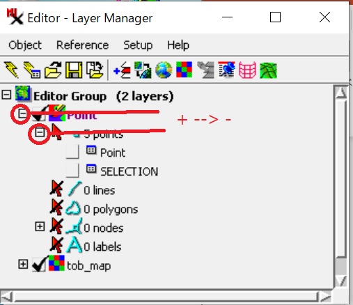
Open “Edit”

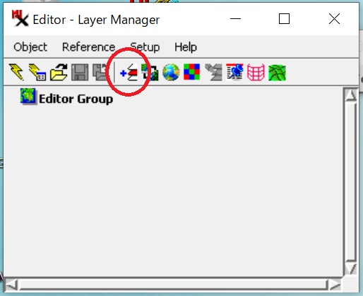
「Editor – Layer Manager」

In Layer Manager,

Push +Mark Symbol (Add reference object)

Select object to display

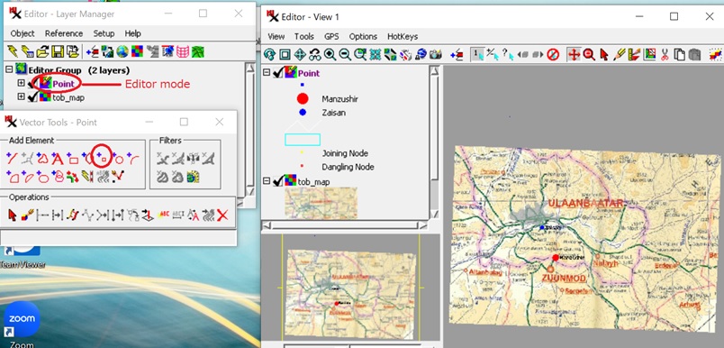
「Editor View and Layer Manager」

Select file and then select objects (raster style map) and vector object (new).

Push OK, then open “Layer Manager” and “Editor – View”

In Layer Manager, Select “vector object” and push a pencil mark button.

“Vector Tools – Point” appears.

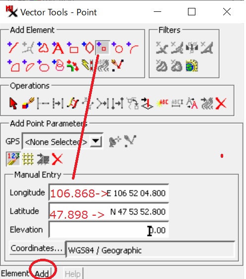
In “Add Element”, select point (⁺□).

In case of having GPS data, Input coordination data in “Add Point Parameters”.

Put data into Longitude and Latitude (decimal). Then push “Add”.

For example,

Plant3 (2017, G4 206): 47_53_55.4, 106_52_01.9 pH 6.76, EC 28.9, Ca 52.2, NO3 7.2

Latitude:47+53/60+55.4/3600

=47.883+0.015=47.898,

Longitude:106+52/60+1.9/3600

=106.867+0.001=106.868

In case of having no GPS data, use Manual Entry.

Push allow mark (↖).

Cross mark (+) should be on the point in the map.

Then push “Add”.

Input data

Input data in a table

In Editor-Layer Manager

Push “+” of the object

(+) (Vector object mark)

(+)Points

Lines

Polygons

Nodes

Labels

Push “+” of points

Creation of New Table

Click the square point (- ↖　■ 5points)

Menu｛Mark All ・・・ New Table ・・｝

Select New Table

User Defined、Next

Input Name of a table, e.g., GEO. Next.

Data Select “Exactly one record for each element”, Next, Finish.

Table Properties

Table

Field

Add new field (Yellow sandwich shape)

Open new field

Input style, select Unicode.

Add data space.

Push next table mark「✔」, then Table appears.

Push “Arrow mark” for the new point in the Editor View.

Input data of the new point.

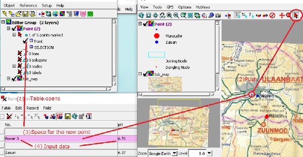
Showing

Data symbol (size and color) is shown automatically on the map.

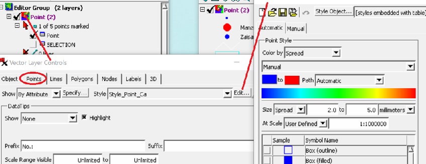
You can modify style. Push the object mark in the layer manager.

“Vector Layer Control”

Menu: Object Points Lines Polygons Nodes Labels 3D

Select “Points”/ Show {By Attribute}/ Select by Attributes or New one.

For example, Color by “spread”. Size “spread”, “2.0” to “5.0” millimeters.

Size is shown in the map scale, for example, at scale “User defined”, “1:1000000”.

To top (Link)

=====================